Representation learning has been widely used and studied in CV&NLP. It is not surprising that people transfer the methods and ideas to reinforcement learning, especially for generalization and data-efficiency.
SimCLR, as a widely used self-supervised learning (SSL) method, has achieved excellent performance in CV tasks. The very basic idea is to learn a representation. Under ideal circumstances, representations of pictures are high-level information abstract. SimCLR forces the representation network to learn invariants among pictures with a carefully designed structure.
    graph LR
id1[pic]
id2[aug1]
id3[aug2]

id1--->id2
id1--->id3

id4[repre]
id5[repre]

id2-->id4
id3-->id5

id6[proj1]
id7[proj2]

id4-->id6
id5-->id7
In this graph, aug indicates augmentation, repre indicates representation and proj indicates projection.
The high-level idea is that for 2 augmentations generated by a single picture, the objective of the representation network is to maximize their similarity. This idea is called contrastive learning. So one picture is augmented by the same method, random crop for example, to generate 2 augmented pictures. Then the augmented pictures are processed by the representation network. Finally, we project the representations into a lower-dimension space (projection space) and update the network to maximize target similarity.
Let’s have a closer look. We can easily define how similar two pictures are. A common way is cosine similarity. $$sim(pic_1,pic_2) = \frac{pic_1\cdot pic_2}{||pic_1||\cdot ||pic_2||}$$
So how do we utilize this similarity definition and turn it into a loss? SimCLR uses a contrastive learning loss called NT-Xent loss (Normalized Temperature-Scaled Cross-Entropy Loss). Yes, a pretty long name😅. One thing to notice is that augmentations from the same source are naturally matched and to be ‘pulled together’. Therefore, the first thing we do is to calculate the probability that ’two augmented pictures are from the same source’. We do this with the softmax function. $$softmax=\frac{e^{sim(pic_1,pic_2)}}{\sum e^{sim(\text{other augmented pic pairs, regardless of source picture})}}$$ The objective aims to make the value of softmax above as large as possible, so we take a negative log. $$l(pic_1,pic_2) = -log(softmax)$$ Then we calculate the same value for interchanged pair $l(pic_2,pic_1)$.
The final loss is the average of all pairs & interchanged pairs’ $l$ loss over the batch. $$L = \frac{l(pic_1,pic_2) + l(pic_2,pic_1) + l(pic_3,pic_4) + l(pic_4,pic_3) \dots}{1+1+\dots}$$ where $pic_3\ pic_4$ are from another source picture.
Noted that there’s only one representation network and only one projection network. After well-training the representation, we can use them for down-stream tasks, for example classification.
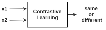
It seems like the method is still promising if we transfer it to RL scenario, replacing all pictures by states/observations. Is it true? Obviously, no, otherwise PSM does not need to exist😁. The problem is that states in RL settings cannot be naturally matched. We can hardly tell that state-1 from trajectory-1 should be matched with state-2 in trajectory-2 since states’ relation is not as obvious as ’they are from the same source picture’. We need a metric to describe how close 2 states are.
PSM is designed to solve the problem, and the high-level idea is that ‘optimal policy chooses similar actions in similar states’. In other words, the similarity between states is the behavioral similarity between optimal trajectories. The distance between states is measured by the bisimulation metric in PSM paper.
Bisimulation metrics, at the very beginning, are proposed to compress super large or continuous MDPs. It’s a definition to measure how bisimilar 2 states are. Basically, it consists of 2 parts: the difference in immediate reward for the same action and the difference in probability of transferring into the same class of states. What does PSM do? PSM first abandoned the reward term since the reward does not provide any helpful information about behavior. PSM measures the difference in immediate action with a certain distance and the difference in transition probability with Wasserstein-1 distance. $$d^*(x,y)=\text{DIST}(\pi^*(x),\pi^*(y))+\gamma W_1(d^*)(P^{\pi^*}(\cdot|x),P^{\pi^*}(\cdot|y))$$ We can see this is a recursive definition and can be computed via dynamic programming. Then we can learn a representation with the following process:
    graph LR
id3[state1,...]
id4[state1',...]
traj1-->id3
traj2-->id4
id5[Compute state similarity]
id3-->id5
id4-->id5
id6[Match with SimCLR for most similar pair]
id5-->id6
This is my very first time writing a relatively long blog in English, and if there is any problem, pls let me know. Thanks for reading😁