Data-Efficient Reinforcement Learning with Self-Predictive Representations
As we see in the blog, policy similarity metric (PSM) uses a specially designed bisimulation relation to force representation network to learn the transition dynamics. This blog will give a brief overview of another method, self-predictive dynamics, which learns about transition dynamics in a more explicit way.
The goal of SPR is to improve the sample-efficiency with self-supervised process. This leverages limitless training signals from self-predictive process. The very high level idea is: the representation component of the architecture will predict a piece of future trajectory, then we minimize the gap between predicted future state and the real future state. The trained representations will be later fed to q-learning head as the input of Rainbow. Intuitively, the representation is forced to understand the environment dynamic.
Let’s have a closer look.
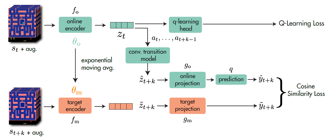 As you can see, the architecture consists of 4 major parts and a RL head. Namely: the online encoder, the target encoder, the convolutional transition model and the projections. We will see each part in detail.
Online Encoder: online encoder $f_o$ transforms observed state $s_t$ into representation $z_t:=f_o(s_t)$.
Target Encoder: target encoder $f_m$ is very similar to the online one, but it’s not a ’trained’ network and will not be updated with back-propagation. The target encoder computes the representation of future states via exponential moving average (EMA): denote parameters of $f_o$ as $\theta_o$, parameters of $f_m$ as $\theta_m$, the EMA rule is: $$\theta_m \leftarrow \tau \theta_m + (1-\tau) \theta_o$$
Conv. Transition Model: the convolutional transition model is an action-conditioned model. Its function is to generate a sequence of $K$ predictions for $\tilde{z_{t+1:t+K}}$. We compute $\hat{z_{t+k+1}}:=h(\hat{z_{t+k}},a_{t+k})$ iteratively starting from $\hat{z_t}:=z_t:=f_o(s_t)$. We then compute the ‘real’ representations $\tilde{z_{t+1:t+K}}$ with $f_m$ and $s_{t+1:t+K}$. The actions and $s$s are sampled from ‘real’ interactions.
Projection: 2 projection heads are used: online projection head $g_o$ and target projection $g_m$. They project the representations into a smaller latent space. Notice that, there’s a additional prediction head $q$ applied to online projections to predict the target projection. $$\hat{y_{t+k}}:=q(g_o(\hat{z_{t+k}}))$$
$$\tilde{y_{t+k}}:=g_m({\tilde{z_{t+k}}})$$
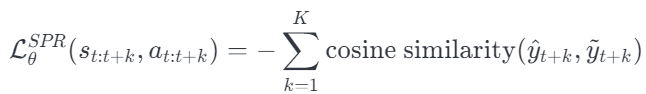
After constructing all projections required, we compute the self-predictive loss by summing up all minus-cosine-smiliarity of all time steps in (t+1) to (t+K)
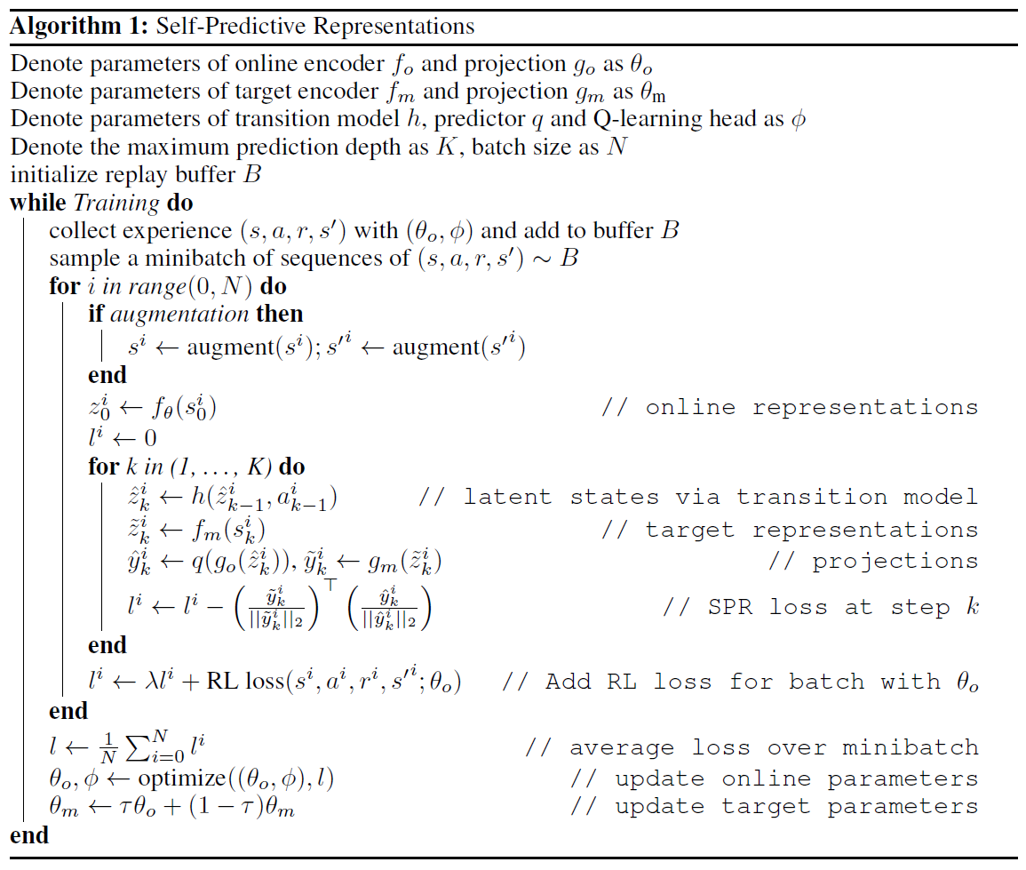
The SPR loss is integrated into the RL loss as an aux loss. And the algorithm is like the following:
Given the paper’s intense discussion about implementation detail and choices of hyperparameters, methods & design, it might be a hard-to-train algorithm. Compared with other works which simply transfer SSL/RepreL methods to RL, the paper fully consider the sequential property of RL problems, which seems to be promising.