References:
Tutorial on Diffusion Models for Imaging and Vision by Stanley Chan
Dr. Yang Song’s blog on Score Matching
Basics of Langevin Dynamics
Unlike DDPM, which models the generative model as a hidden variable model with $x_{1:T}$ as the hidden variables, score-matching models, while deeply linked to DDPM, starts from a sampling view and later concerns about the distribution we sampled from. Let’s start with an assumption that we have a distribution $p(x)$ that we can sample from, and this distribution is exactly the distribution we want (say, the image distribution of a cat).
The Langevin Dynamics saples data from an iterative procdure, with $t=1,2,3,…,T$: $$ x_{t+1} = x_t + \tau \nabla_x \log p(x_t) + \sqrt{2\tau}z,\quad z\sim \mathcal{N}(0, I) $$
If ignored the noise term $\sqrt{2\tau}z$, the Langevin Dynamics is exactly the gradient decent of the log-likelihood of the data. The decent direction $\nabla_x \log p(x_t)$ makes the data converge to distribution $p(x)$.
Another way to think of this is to consider the $x$ to be a peak of a hill (like the tip of a Gaussian distribution), and the $\nabla_x \log p(x_t)$ is the force that pushes the $x$ to the bottom of the hill. So the Langevin Dynamics is equivalent to: $$ x^\star = \argmax_x \log p(x) $$
Notice that the distribution is fixed, but we move around with $x$ to find t he peak of the distribution.
After we have the regular gradient decent, we add a noise with fixed step size $\sqrt{2\tau}z$ to the $x$ to make the sampling go around and oscillate around the peak. In this view, Langevin dynamics is stochastic gradient decent.
Stein’s Score Function
In the previous section, the distribution $p(x)$ is assumed to be fixed. Now we parametrize the distribution with a parameter $\theta$, and the distribution becomes $p_\theta(x)$.
The Stein’s score function is defined as: $$ s_\theta(x) \triangleq \nabla_x \log p_\theta(x) $$
Do not confuse with ordinary score function which is about $\theta$: $$ s_x(\theta) = \nabla_\theta \log p_\theta(x) $$
Now we call Stein’s score function as the score function.
The score function is the gradient w.r.t. $x$. It is a vector field, and we can see from a 2-D example: $$ \nabla_x \log p_\theta(x) = \begin{bmatrix} \frac{\partial}{\partial x_1}\log p_\theta(x) \\ \\ \frac{\partial}{\partial x_2}\log p_\theta(x) \end{bmatrix} $$
Edited & Updated on Sep 4th 2024
Score Matching for Generative Models
Having some idea about the score function, we can now take a look at 2 papers by Dr. Yang Song from Standford and OpenAI. The first one is Generative Modeling by Estimating Gradients of the Data Distribution. We will take a score-based model perspective instead of the traditional diffusion model view in this blog series(but we will soon see that they are deeply connected).
Generative Modeling by Estimating Gradients of the Data Distribution
Before focusing on the score matching, the big picture is that we want to model the data distribution $p(x)$ and sample new data out of it. In likelihood-based models, we directly model the PDF with parameters. The PDF looks like
$$ p_\theta(x) = \frac{1}{Z(\theta)}\exp(f_\theta(x)) $$
where $Z(\theta)$ is viewed as a normalizing constant such that $\int p_\theta(x)dx = 1$. The $f_\theta(x)$ is the energy function (unnormalized probalistic model), and the $Z(\theta)$ is the partition function. During training, we do following optimization problem: $$ \max_\theta \sum_{i=1}^N \log p_\theta(\mathbf{x}_i) $$
which is nothing but the maximum log-likelihood estimation. However, it is hard to compute the partition function $Z(\theta)$, which is the integral of the energy function over the whole space.
To avoid computing $Z(\theta)$, we can model score function instead. The score function, again, is $\nabla_x \log p_\theta(x)$. We learn $s_\theta(x)\approx \nabla_x \log p_\theta(x)$ instead of $p_\theta(x)$. We now get rid of the partition function $Z(\theta)$!
Fisher divergence is used to measure the difference between the true score function and the estimated score function. The Fisher divergence is defined as $$ D_F(s_\theta, \hat{s}_\theta) = \mathbb{E}_{x\sim p(x)}\left[|s_\theta(x) - \hat{s}_\theta(x)|^2\right], \quad \hat{s}_\theta(x) = \nabla_x \log p_\theta(x) $$
The Fisher divergence still require some knowledge about the unknown data score as the ground truth. There are several ways to overcome this. One simplest way is to assume a distribution of the data, called Explicit Score-Matching.
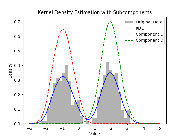
Explicit Score-Matching employs classical kernal density estimation (KDE), which is a non-parametric method to estimate the data distribution. Given the data $\mathbf{x} = {x_1, x_2, …, x_N}$, the data distribution is estimated as $$ \hat{p}(x) = \frac{1}{N}\sum_{i=1}^N k(x - x_i) $$
where $k(\cdot)$ is the kernel function. I made a sample plot for 1-D data sampled from 2 Gaussian distributions. The kernel density estimation is shown below.
Given the data is known, and the model is known, we have access to the ground truth score function. We can do score-matching explicitly: $$ J_{\text{ESM}}(\theta) := \mathbb{E}_{x\sim \hat{p}(x)}\left[|s_\theta(x) - \nabla_x \log \hat{p}(x)|^2\right] $$
By substituting the expectation with the weighted sum, we have: $$ \begin{aligned} J_{\text{ESM}}(\theta) &= \sum_{i=1}^N w_i|s_\theta(x_i) - \nabla_x \log \hat{p}(x_i)|^2 \\ & = \sum_{i=1}^N w_i|s_\theta(x_i) - \nabla_x \log \left(\frac{1}{N}\sum_{j=1}^N k(x_i - x_j)\right)|^2 \\ & = \sum_{i=1}^N \hat{p}(x) |s_\theta(x_i) - \nabla_x \log \left(\frac{1}{N}\sum_{j=1}^N k(x - x_j)\right)|^2 \end{aligned} $$
Then we can optimize. After optimization, we use the Langevin dynamics to sample from the model distribution: $x_{t+1} = x_t + \tau \nabla_x \log p_\theta(x_t) + \sqrt{2\tau}z$. For this method, the bad news is that the KDE is so bad that it cannot capture complex data distribution.
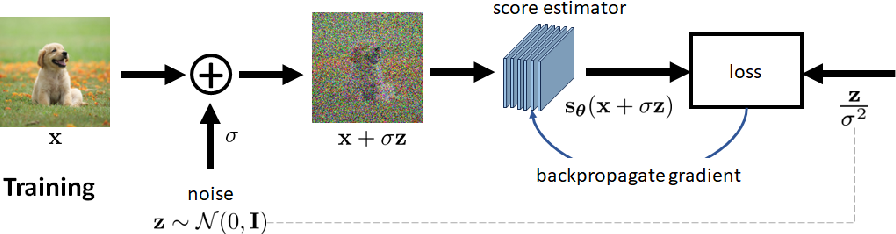
Denoising Score Matching(DSM) is a better way to estimate the score function. As you can tell from the name, it connects to diffusion models! Previous works suggest that the objective function for DSM is: $$ J_{\text{DSM}}(\theta) = \mathbb{E}_{q(x, x’)} \left[\frac{1}{2}|s_\theta(x) - \nabla_x q(x|x’)|^2\right] $$
We access the ground truth score function by conditional distribution instead of a fixed estimation like KDE. Here the trick is, we don’t know the ground truth distribution/score function at all. But if we make $x$ a noisy version of $x’$, it is easier for us to get the ground truth score function. What’s more, if the noising version is controlled by us, say $x = x’ + \sigma z$, we can estimate $q(x|x’)$ by the Gaussian distribution! The $q(x|x’)$ is the conditional distribution of $x$ given $x’$, and it is a Gaussian distribution with mean $x’$ and variance $\sigma^2$.
$$ \begin{aligned} \nabla_x \log q(x|x’) &= \nabla_x \log \mathcal{N}(x; x’, \sigma^2) \\ &= - \frac{x - x’}{\sigma^2} \end{aligned} $$
Plug this into the objective function, we have: $$ \begin{aligned} J_{\text{DSM}}(\theta) & = \mathbb{E}_{q(x, x’)} \left[\frac{1}{2}|s_\theta(x) + \frac{x - x’}{\sigma^2}|^2\right]\\ & = \mathbb{E}_{q(x’)} \left[\frac{1}{2}|s_\theta(x’ + \sigma z) + \frac{z}{\sigma^2}|^2\right]\\ \end{aligned} $$
Prof. Stanley Chen from Purdue Univ has a great picture illustrating DSM:
One other way to understand DSM’s objectiv is through the equivalence between DSM and ESM, i.e. $J_{\text{DSM}}(\theta) = J_{\text{ESM}}(\theta) + C$. The proof is in the paper Vincent 2011.
Other ways to do score-matching. There are many other ways to do score-based generation. Despite what we have discussed about, one may want to take a look at Sliced Score-Matching.
Better Score-Matching Models
As claimed by Yang Song, estimated score functions are inaccurate in low-density regions. In the loss function of ESM we can see, $\int p(x) |s_\theta(x) - \nabla_x \log p(x)|^2 dx$ is weighted by $p(x)$. In low-density regions, the $p(x)$ is small, and the loss is not well optimized.
When sampling from the langevin dynamics, we are likely to sample from low-density regions. The score function is inaccurate in low-density regions, and the resulting sampling will not be good.
Score-based generative modeling with multiple noise perturbations
One way proposed by Yang Song is to perturb the data with multiple noise levels. Data perturbed by different noise levels will cover those low-density regions.
Now we have a problem. Strong noise perturbation will make the data far from the original data distribution. We need to balance the noise level. The noise level is controlled by the variance of the Gaussian distribution. We can use a series of increasing variance to perturb the data: $\sigma_1, \sigma_2, …, \sigma_K, \sigma_{i}\leq \sigma_{i+1}$.
We can construct a new data distribution (actually multiple distributions with different noise level) with the perturbed data: $$ p_{\sigma_i}(x) = \int p(y)\mathcal{N}(x; y, \sigma_i^2 I)dy $$
where $p(y)$ is the original data distribution. To sample from such a distribution, we sample $x \sim p(x)$ and $x + \sigma_i z$ where $z\sim \mathcal{N}(0, I)$.
Using a Noise Conditional Score-Based Model $s_\theta(x, i)$, we hope to approximate the score function of the perturbed data distribution such that $s_\theta(x, i) \approx \nabla_x \log p_{\sigma_i}(x)$ for all $i$. The loss function is then a weighted fisher divergence: $$ \sum_{i=1}^K \lambda(i)\mathbb{E}_{x\sim p_{\sigma_i}(x)} (\text{Matching Loss at } i) $$
Of course, the matching loss is $|s_\theta(x, i) - \nabla_x\log p_{\sigma_i(x)}|^2$. The $\lambda(i)$ is the weight for each noise level. The $\lambda(i)$ is a hyperparameter and often chosen to be $\sigma_i^2$ (the larger the noise level, the more weight it has).
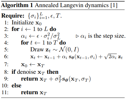
In conventional score matching, we directly sampling along the direction of score function (Langevin Dynamics). In this new model, we sample along the direction of the perturbed score function. Which is annealed Langevin dynamics.
There are several tricks in training & sampling with perturbed data distribution. One might refer to Improved Techniques for Training Score-Based Generative Models.
Bridging Score Matching and Stochastic Differential Equations
Stochastic Calculus is hard. But we might just view it as some stochastic process in a fancy formalism.
Here is a basic generic form of SDE: $$ dx = f(x, t)dt + g(t)dw $$
where $f(x, t)$ is the drift term, $g(t)$ is the diffusion term, and $dw$ is the Wiener process. The solution to this SDE is a stochastic process $x(t)$. If we let $p_t(x)$ be a function of $x(t)$, then it is analogous to $p_{\sigma_i}(x)$ in the previous section. $p_0(x)$ is the original data distribution.
If we mess the SDE for a long time and let $t\to T$, the solution $x(t)$ will converge to a stationary distribution $p_T(x)=\pi(x)$, called prior distribution.
So as you may see, SDE’s process is similar to perturb data step-by-step increasing the perturbation level.
To sample from the SDE above, we can use the reverse SDE. It exists for any SDE. The reverse SDE is defined as: $$ dx = \left[-f(x, T-t) + \frac{1}{2}g^2(T-t)\nabla_x\log \pi(x)\right]dt + g(T-t)dw $$
Or we can have the better form with $t$ to be negative: $$ dx = \left[f(x, t) + \frac{1}{2}g^2(t)\nabla_x\log \pi(x)\right]dt + g(t)dw $$
As you may have found, the reverse SDE contains the score function $\nabla_x\log \pi(x)$.
To solve the reverse SDE, we first need to know what is the definition of the solution. A solution to a SDE is a stochastic process $x(t)$ that satisfies the SDE. To solve, we have to know terminal condition $p_T(x)$, which in our case is the prior distribution $\pi(x)$. We also have to know the score function $\nabla_x\log \pi(x)$, and we train the model to approximate this score function.
Training the Score Function in SDE Framework
Recall our objective function in perturbed data distribution: $$ \sum_{i=1}^K \lambda(i)\mathbb{E}_{x\sim p_{\sigma_i}(x)} (\text{Matching Loss at } i) $$
We can rewrite the matching loss as: $$ \mathbb{E}_{t\sim \text{Uniform}(0, T)}\mathbb{E}_{p_t(x)}\left[\lambda(t)\cdot\text{Matching Loss at } i\right] $$
Quite similar huh? The $\lambda(t)$ is the weight for each time step. The $\lambda(t)$ is a hyperparameter used to balance the magnitude of different score matching losses.
Once the score function is well-trained (say by denoising score matching), we can sample from the reverse SDE to get samples from the prior distribution $\pi(x)$ (just plug the score function into the reverse SDE, and continuously push $t$ to $T$).
Likelihood weighting function. Song mentioned a special case in his blog, that when the drift term $f(x, t)$ is $\lambda(t) = g(t)^2$, there is a connection between KL divergence between $p_0$ and $p_\theta$ and the weighted Fisher divergence.
$$ \begin{aligned} \text{KL}(p_0(x)|p_\theta(x)) &\leq \\ &\frac{T}{2}\mathbb{E}_{t \in \mathcal{U}(0, T)}\mathbb{E}_{p_t(x)}[\lambda(t) | \nabla_x \log p_t(x) - \mathbf{s}_\theta(x, t) |_2^2] + \text{KL}(p_T \mathrel| \pi) \end{aligned} $$
Solvers for Reverse SDE
One way to solve Euler-Maruyama method. The Euler-Maruyama method is a numerical method to solve SDE. The method is simple: we discretize the time $t$ into $T$ steps, and at each step, we sample from the Gaussian distribution and update the $x$.
$$ \begin{aligned} x_{t+1} &= x_t + f(x_t, t)\Delta t - g^2(t)s_\theta(x,t)\Delta t + g(t)\sqrt{|\Delta t|}z_t \\ z_t &\sim \mathcal{N}(0, I) \\ \Delta t &= \frac{1}{T} \end{aligned} $$
There are other SDE solvers can be applied, we skip the details here.
Conclusion
In this blog, we have discussed the basics of Langevin Dynamics, Stein’s score function, and score matching. We have also discussed the connection between score matching and SDE. The core part of this blog is how we train the score function, and how we apply score-matching techniques to SDE framework. We will discuss more about the sampling and ODEs in the next blog.