- A Glimpse of Differential Equations
- Constructing Training Targets for Flow & Diffusion Models from DE View
- Actually Optimizing for the Target Constructed
- A Summary on Both Models from Differential Equations View
- References
A Glimpse of Differential Equations
We can view the target objects as vectors $z\in \mathbb{R}^d$, which is reasonable this notation is enought for many cases like images, videos or robots’ actions.
To generate an object well, we look for the object is likely under the desired distribution. Formally, we have distribution of data $p_{data}:\mathbb{R}^d\to \mathbb{R}_{\geq 0}$, and $z\sim p_{data}$, we want to sample $z$ from $p_{data}$. That’s what we mean by saying generating something. Moreoever, we have $z_1, z_2, \cdots, z_n\sim p_{data}$ in practice as our dataset. If the generation is conditional, say we want a dog picture instead of random animal picture, we have $z\sim p_{data}(\cdot|y)$, where $y=\text{a dog picture}$ is the condition.
Flow Models
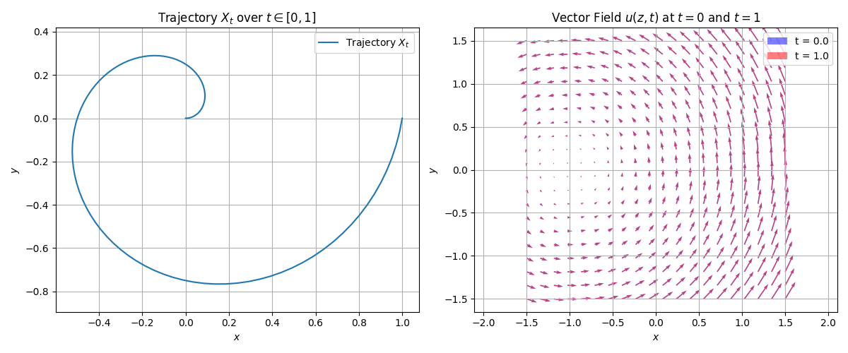
A trajectory is a function of time $X: [0, 1]\to \mathbb{R}^d, t\to X_t$.
A vector field is $u: \mathbb{R}^d \times [0, 1]\to \mathbb{R}^d, (z, t)\to u(z, t)$.
An ODE (Ordinary Differential Equation) have $X_0=x_0$ which is the initial condition, and $$\frac{dX_t}{dt} = u_t(X_t), \quad t\in [0, 1]$$.
There are many different trajectories $X_t$ for different initial conditions $x_0$. We collect them together and call them a flow.
$$\psi:\mathbb{R}^d \times [0, 1]\to \mathbb{R}^d, (x_0, t)\to \psi_t(x_0)$$
where $\psi_t(x_0)=x_0$ is the trajectory starting from $x_0$ at time $t=0$, and $\frac{d\psi_t(x_0)}{dt} = u_t(\psi_t(x_0))$ is the ODE. In simple words, a flow $\psi(x_0)$ gives the pposition at time $t$ of the trajectory starting from $x_0$ at time $t=0$. Once $x_0$ is given, the flow $\psi(x_0)$ is a function of time.
That is, a vector field defines a ODE, and a flow is the solution of the ODE.
Example: Linear ODE
Simple vector field $u_t(x) = -\theta x$ where $\theta>0$. The ODE is $\frac{dx_t}{dt} = -\theta x_t$, and the solution is $x_t = e^{-\theta t}x_0$. The flow is given by $\psi_t(x_0) = e^{-\theta t}x_0$.
However, most of the time we don’t know the solution as in the above example. We can use a numeircal method to simulate the ODE. For example, we can use Euler’s method to discretize the ODE, which is moves a bit in the direction of the vector field at each timestep, and we returen the final trajectory.
Recall our goal is to transform $p_{init} \to p_{data}$, where $p_{init}$ is the distribution of the initial condition $x_0$. We can use an ODE to do this. We use a neural network to represent (and learn) the vector field.
$$u_t^\theta:\mathbb{R}^d \times [0, 1]\to \mathbb{R}^d$$
We sample random initial conditions $x_0\sim p_{init}$, and we use the ODE $$\frac{dx_t}{dt} = u_t^\theta(x_t)$$ to simulate the trajectory $x_t$ for $t\in [0, 1]$. In ideal case, the end point $x_1$ is distributed as $p_{data}$. The Euler’s method in this case can be used to generate.
If Adding Stochasticity to the Differential Equations
For a stochastic process, we have $X_t$ as a random variable and $X:[0,1]\to \mathbb{R}^d, t\to X_t$ is a stochastic process. If we run the process twice, we get two different trajectories.
The vector field for SDE is $u_t:\mathbb{R}^d \times [0, 1]\to \mathbb{R}^d, (z, t)\to u(z, t)$, and the SDE is given by the stochastic differential equation (SDE) as follows: $$dX_t = u_t(X_t)dt + \sigma_t dW_t$$
where $W_t$ is a standard Wiener process (Brownian motion). The first term is the drift term, and the second term is the diffusion term. The drift term is deterministic, and the diffusion term is stochastic. We therefore introduced stochasticity to the ODE. Similar to the ODE, we can simulate the SDE using Euler-Maruyama method, which is a numerical method for simulating SDEs. The Euler-Maruyama method is given by the following equation: $$X_{t+h} = X_t + u_t(X_t)h + \sigma_t\Delta W_t$$
where $\Delta W_t$ is the increment of the Wiener process, which is a random variable with mean 0 and variance $h$. The increment $\Delta W_t$ is independent of $X_t$.
A $dX_t$ Notation
Trajectory ODE $\frac{dX_t}{dt} = u_t(X_t)$ is equivalent to $X_{t+h} = X_t + hu_t(X_t) + hR_t(h)$, where $\lim_{h\to 0}R_t(h)=0$. The $dX_t$ notation is a shorthand for the above equation. The $dX_t$ notation is used in SDEs to denote the infinitesimal change in the trajectory.
Side Note: SDEs are quite useful as well in terms of quantitative trading. For example, the Ohrnstein-Uhlenbeck process is a stochastic process that is used to model the mean-reverting behavior of asset price gap (spread).
Constructing Training Targets for Flow & Diffusion Models from DE View
Recall that our goal is to transform $X_0\sim p_{init}$ with $dX_t=u_t^\theta(X_t)dt$ to $X_1\sim p_{data}$. That mean we need to have a meaningful vector field $u_t^\theta$ by training $\theta$.
One of the most natural form of trianing target is: $$ L(\theta)=||u_t^\theta(x) - u_t^{target}(x)||^2 $$
The question is: how to get the target vector field $u_t^{target}(x)$? We have seen in previous posts in diffusion family using score matching, and we can get the training target from differential equations’ view.
Conditional and Marginal Distribution Path
Consider a Dirac distribution: $z\in \mathbb{R}^d, \delta_z, X\sim \delta_z \Rightarrow X=z$. The Dirac distribution is a distribution that is concentrated at a single point.
We define the conditional probability path: $p_t(\cdot|z)$, it has several properties:
- $p_t(\cdot|z)$ is a probability distribution over $\mathbb{R}^d$.
- $p_t(\cdot|z)$ is a Dirac distribution $\delta_z$ at $z$ when $t=1$.
- $p_t(\cdot|z)$ is a $p_{init}$ distribution when $t=0$.
We can look at the example of a Gaussian probability path, where $p_t(\cdot|z) = \mathcal{N}(\alpha_t z, \beta_t^2 I_d)$, where $\alpha_t$ and $\beta_t$ are the parameters of the Gaussian distribution. The $\alpha_t$ starts at 0 and ends at 1, and $\beta_t$ starts at 1 and ends at 0. The Gaussian probability path is a continuous path that connects the Dirac distribution at $z$ to the $p_{init}$ distribution.
This is a conditional probability path because it has a condition on $z$ and it collapses to a Dirac distribution concentrating at $z$ when $t=1$.
We define a marginal probability path: $z\sim p_{data}, X\sim p_t(\cdot|z)\Rightarrow X\sim p_t$, where $p_t$ is the marginal distribution. The marginal distribution is a probability distribution over $\mathbb{R}^d$ that is obtained by integrating out the condition $z$. Therefore we get rid of the condition $z$. Similarly it has several properties:
- $p_t(x)=\int p_t(x|z)p_{data}(z)dz$ is a probability distribution over $\mathbb{R}^d$. This is similar to the marginalizing method in Bayesian networks.
- $p_0=p_{init}, p_1=p_{data}$.
Conditional and Marginal Vector Field
If we consider each data point in the data space, we can define a vector field $u_t^{target}(x|z), 0\leq t \leq 1, x,z\in \mathbb{R}^d$.
So what does it do? Previously we have seen a probability path that changes from $p_{init}$ to $\sigma_z$ throught the transformation of $p_t(\cdot|z)$. We want to find a ODE such that we can follow its vector field to get a point from $p_{init}$ to $p_{data}$. Formally we say the vector field needs to satisfy the following condition:
$$ X_0\sim p_{init}, \frac{d}{dt}X_t = u_t^{target}(X_t|z)\Rightarrow X_t\sim p_t(\cdot|z)\\ p_{init}=p_0, p_{data}=p_1 $$
Let’s look at our Gaussian probability path example. The vector field is given by the following equation: $$u_t^{target}(x|z) = (\dot{\alpha}_t -\frac{\dot{\beta}_t}{\beta_t}\alpha_t)z+\frac{\dot{\beta}_t}{\beta_t}x$$
Notice that we have $z,x\in \mathbb{R}^d$, so we can consider the vector field as a recipe that helps us to find the direction and velocity to move from $p_t(\cdot|z)$ to $p_{t+\Delta t}(\cdot|z)$. And it is like a weighted average between 2 points! (we have some glithches in the GIF due to numerical simulation 😶)
In the same way as before, we have marginal vector field given by: $$u_t^{target}(x) = \int u_t^{target}(x|z)\frac{p_{data}(z) p_t(x|z)}{p_t(x)}dz$$
You might notice a wierd ratio here $\frac{p_{data}(z) p_t(x|z)}{p_t(x)}$. This is a posterior distribution of $z$ given $x$ at time $t$. This is a conditional distribution of $z$ given $x$ at time $t$.
This vector field satisfies:
- $x_o \sim p_{init}, \frac{d}{dt}X_t = u_t^{target}(X_t)\Rightarrow X_t\sim p_t$.
- $p_{init}=p_0, p_{data}=p_1$.
Side Note: Continuity Equation
Given $X_0\sim p_{init}$, $\frac{d}{dt}X_t = u_t^{target}(X_t)$, the following probability path $X_t\sim p_t\ (0\leq t \leq 1)$ is equivalent to the holding of the continuity equation: $$\frac{d}{dt}p_t(x) + \nabla_x (u_tp_t)(x)=0$$. This helps to prove the marginal vector field formula above.
Extending to Stochastic Differential Equations
We can extend the above vector field to SDEs. That is called score function we studied in the previous post!
Still, we consider the single data point first (conditional) and then the general case (marginal). The conditional score is denoted by $\nabla_x\log p_t(x|z)$, and the marginal score is denoted by $\nabla_x\log p_t(x)$.
Recall one of the most powerful formula in ML: $$\nabla_x \log p(x) = \frac{1}{p(x)}\nabla_x p(x)\quad\text{, by chain rule}$$
We know: $$ \begin{aligned} \nabla \log p_t(x|z) &= \frac{1}{p_t(x|z)}\nabla p_t(x|z) \\ &= \frac{1}{p_t(x)}\int \nabla p_t(x|z)p_{data}(z)dz \quad \text{, marginalize}\\ &= \int \nabla \log p_t(x|z) \frac{p_t(x|z)p_{data}(z)}{p_t(x)}dz \\ \end{aligned} $$
For marginal and conditional score, we are both taking the gradient w.r.t. $x$.
Now, you might be wondering why do we introduce score here? The reason is that we can use the score function convert ODE target to SDE. Firtly, it is related to the ODE.
Consider our previous Gaussian probability path example. Viewing from the probability path view, the transformation is given by: $$ p_t(\cdot|z) = \mathcal{N}(\alpha_t z, \beta_t^2 I_d)\\ $$
The vector field is given by: $$u_t^{target}(x|z) = (\dot{\alpha}_t z -\frac{\dot{\beta}_t}{\beta_t}\alpha_t)z+\frac{\dot{\beta}_t}{\beta_t}x$$
For the score function, we have already known the $p_t(x|z)$ (because we designed it), and we can plug into the formula: $$ \nabla_x \log p_t(x|z) = -\frac{x-\alpha_t z}{\beta_t^2} $$
Theorem: SDE Extension Trick
Let $u_t^{target}(x)$ be as before, then for aribitrary diffusion coefficient $\sigma_t\geq 0$: $$ \begin{aligned} X-0\sim p_{init},\ &dX_t=[u_t^{target}(X_t)+\frac{\sigma_t^2}{2}\nabla_x\log p_t(X_t)]dt+\sigma_t dW_t\\ &\Rightarrow X_t\sim p_t(x)\\ &\Rightarrow X_t\sim p_{data} \text{, if } t=1\\ \end{aligned} $$
We have the noise term, and we have the original old vector field, and we have the correction term $\frac{\sigma_t^2}{2}\nabla_x\log p_t(X_t)$. The correction term is the score function. The score function is a correction term that helps to correct the drift term.
Actually Optimizing for the Target Constructed
Let’s quickly recap what we have in the differential equation space:
- Flow models are deterministic ODEs. The initial conditions are $X_0\sim p_{init}$, and the ODE goes like $dX_t=u_t^\theta(X_t)dt$.
- Diffusion models are stochastic SDEs. The initial conditions are $X_0\sim p_{init}$, and the SDE goes like $dX_t=u_t^\theta(x_t)dt + \sigma_t dW_t$.
We would then discuss 2 major training methods: flow matching and score matching.
Flow Matching!
Flow matching is learning the vector field $u_t^\theta(x)$.
Suppose we have a neural network $u_t^\theta(x)$, parameterized by $\theta$. The goal is to use the neural network to simulate the vector field. If we can do that well, then we can follow the vector field to get a point from $p_{init}$ to $p_{data}$.
The training is given by flow matching loss: $$ L_{fm}(\theta) = \mathbb{E}_{t\sim \text{Uniform}[0,1],z\sim p_{data}, x\sim p_t(\cdot|z)}{||u_t^\theta(x) - u_t^{target}(x)||^2} $$
where we take a datapoint $z$ from our dataset, and we sample it from a probability path conditioned on that datapoint.
However it is very sad that the flow matching loss is intractable. If we look at the $u_t^{target}(x)$, we see: $$ u_t^{target}(x) = \int u_t^{target}(x|z)\frac{p_{data}(z) p_t(x|z)}{p_t(x)}dz $$
This means that we have to integrate over the entire dataspace (e.g. all the images in the world/huge dataset) to get the target vector field. This is intractable.
What we can acutally compute is a conditional flow matching loss: $$ L_{cfm}(\theta) = \mathbb{E}_{t\sim \text{Uniform}[0,1],z\sim p_{data}, x\sim p_t(\cdot|z)}{||u_t^\theta(x) - u_t^{target}(x|z)||^2} $$
We change the target vector field to the conditional vector field. This is tractable. Moreover, we have a theorem indicating the equivalence between the flow matching loss and the conditional flow matching loss, thus the minimizer $\theta^*$ is the same. $$ L_{fm}(\theta) = L_{cfm}(\theta) + C,\ C \geq 0,\ \text{independent of } \theta $$
Example: Gaussian Path
Probability path: $p_t(\cdot|z) = \mathcal{N}(\alpha_t z, \beta_t^2 I_d)$, where $\alpha_t = t$ and $\beta_t = 1-t$.
The vector field is given by: $$u_t^{target}(x|z) = (\dot{\alpha}_t -\frac{\dot{\beta}_t}{\beta_t}\alpha_t)z+\frac{\dot{\beta}_t}{\beta_t}x$$
Suppose we sample a data point $\epsilon\sim \mathcal{N}(0, I_d)$, the we call our $x$ to be $\alpha_t z + \beta_t\epsilon \sim p_t(\cdot|z)$, which is a simple Gaussian distributed point.
We plug the conditional vector field into the flow matching loss, we have: $$L_{cfm}(\theta) = \mathbb{E}_{t\sim \text{Uniform}[0,1],z\sim p_{data}, x\sim p_t(\cdot|z)}[||u_t^\theta(x) - (\dot{\alpha}_t -\frac{\dot{\beta}_t}{\beta_t}\alpha_t)z+\frac{\dot{\beta}_t}{\beta_t}x||^2]$$
Then we replace the $x$ with $\alpha_t z + \beta_t\epsilon$ as a point falls somewhere along the probability path conditioned on $z$. We have: $$L_{cfm}(\theta) = \mathbb{E}_{t\sim \text{Uniform}[0,1],z\sim p_{data}, \epsilon\sim \mathcal{N}(0, I_d)}[\\||u_t^\theta(\alpha_t z + \beta_t\epsilon) -\\ (\dot{\alpha}_t -\frac{\dot{\beta}_t}{\beta_t}\alpha_t)z+\frac{\dot{\beta}_t}{\beta_t}(\alpha_t z + \beta_t\epsilon)||^2]$$
Simplifying the above equation, we have: $$L_{cfm}(\theta) = \mathbb{E}_{t\sim \text{Uniform}[0,1],z\sim p_{data}, \epsilon\sim \mathcal{N}(0, I_d)}[||u_t^\theta(\alpha_t z + \beta_t\epsilon) - (\dot{\alpha}_t z + \dot{\beta}_t\epsilon)||^2]$$
With our setting of $\alpha_t = t$ and $\beta_t = 1-t$, we have: $$L_{cfm}(\theta) = \mathbb{E}_{t\sim \text{Uniform}[0,1],z\sim p_{data}, \epsilon\sim \mathcal{N}(0, I_d)}[||u_t^\theta(t z + (1-t)\epsilon) - (z - \epsilon)||^2]$$
This is also called as conditional optimal transport path.
Score Matching!
Score matching in principles is the same as flow matching.
According to SDE extention trick, we have: $$ dX_t = [u_t^{target}(X_t)+\frac{\sigma_t^2}{2}\nabla_x\log p_t(X_t)]dt+\sigma_t dW_t $$
If we want to simulate the SDE here, we need to construct a score network $s_t^\theta(x)$. We first have the marginal loss (spoiler: it is intractable as well): $$ L_{sm}(\theta) = \mathbb{E}_{t\sim \text{Uniform}[0,1],z\sim p_{data}, x\sim p_t(\cdot|z)}[||s_t^\theta(x) - \nabla_x\log p_t(x)||^2]$$
Conditional score matching loss is called denoising score matching loss: $$ L_{sm}(\theta) = \mathbb{E}_{t\sim \text{Uniform}[0,1],z\sim p_{data}, x\sim p_t(\cdot|z)}[||s_t^\theta(x) - \nabla_x\log p_t(x|z)||^2]$$
We can do the same thing as before by plug in the $x$ with $\alpha_t z + \beta_t\epsilon$, and we have: $$L_{sm}(\theta) = \mathbb{E}_{t\sim \text{Uniform}[0,1],z\sim p_{data}, \epsilon\sim \mathcal{N}(0, I_d)}[||s_t^\theta(\alpha_t z + \beta_t\epsilon) - \nabla_x\log p_t(\alpha_t z + \beta_t\epsilon|z)||^2]$$
For Gaussian probability case, we get the denoising score matching loss: $$L_{sm}(\theta) = \mathbb{E}_{t\sim \text{Uniform}[0,1],z\sim p_{data}, \epsilon\sim \mathcal{N}(0, I_d)}[||s_t^\theta(\alpha_t z + \beta_t\epsilon) + \frac{\epsilon}{\beta_t}||^2]$$
This what we see in the score matching loss in previous posts!
More on Score Matching: What to learn and what not to learn
The key difference between flow matching and SDE-based models is how they treat the vector field (or drift term) during training.
Here is my understanding: Flow matching essentially assumes that we know the conditional vector field $u^{\text{target}}(x|z)$, but the marginal vector field $u^{\text{target}}(x)$ is intractable, so learning this marginal is our objective. In contrast, in SDE-based methods, we only need to learn the score function because our learning starts from a forward SDE that perturbs the data, and we aim to learn the reverse of this SDE. In the reverse process, the drift term is known, and only the marginal score is intractable.
A Summary on Both Models from Differential Equations View
In generative modeling from a differential equations perspective, flow matching and diffusion models approach the transformation from a simple initial distribution to the complex data distribution differently. Flow matching learns an unknown vector field in a deterministic ODE that pushes $p_{\text{init}}$ to $p_{\text{data}}$, while diffusion models use a predefined SDE with a known drift and diffusion to corrupt data and then learn the score function to reverse that process. Notably, even though an SDE reduces to an ODE when the diffusion coefficient is set to zero, the stochasticity in SDEs typically enhances stability and robustness, and the exact transformation remains unknown in practical scenarios, necessitating learned approximations through conditional flow or score matching.
References
[1] On the Mathematics of Diffusion Models by David McAllester arXiv
[2] MIT Computer Science Class 6.S184: Generative AI with Stochastic Differential Equations Lecture 1-3
[3] What are diffusion models? Lil’Log