Implementation really matters when it comes to training Diffusion Models. In this post, we will discuss some tircks, some problems I encountered, coding details and model architectures that avoid awkward failure of noise in noise out.
Our goal is to generate satisfying samples from 2 common datasets: MNIST (easier) and CIFAR-10 (harder).
References:
Lil’Log What are Diffusion Models?
UNet Architecture
UNet is a common architecture for image generation. People in computer vision community has extended it to many different variants, bringing many tricks and advanced blocks like self attention etc. Here we discuss some blocks and tricks that are employed in huggingface’s implementation of DDPM.
Helper Functions
First of all, the helper functions for UNet:
def exists(x):
    return x is not None

def default(val, d):
    if exists(val):
        return val
    return d() if isfunction(d) else d
These are simple but helps simplifying the code. The exists function is used to check if a variable is None. The default function is used to provide a default value (or default function is the object is a function) if the variable is None.
Upsampling and Downsampling Blocks
The UNet is a U-shaped network which involves upsampling and downsampling. We can use 2 functions to define the upsampling and downsampling blocks:
# up/down sample constructor
def Downsample(dim, dim_out=None):
    return nn.Sequential(
        Rearrange("b c (h p1) (w p2) -> b (c p1 p2) h w", p1=2, p2=2),
        nn.Conv2d(dim * 4, default(dim_out, dim), 1)
    )

def Upsample(dim, dim_out=None):
    return nn.Sequential(
        nn.Upsample(scale_factor=2, mode="nearest"),
        nn.Conv2d(dim, default(dim_out, dim), 3, padding=1)
    )
The Downsample function takes the input dimension dim and output dimension dim_out as arguments. The rearange function is used to rearrange the tensor to the desired shape. For example, if the input tensor is of shape (b, c, h, w), the rearange function will reshape it to (b, c, h/2, w/2), and the channel dimension is multiplied by 4 so the ultimate shape is (b, c*p1*p2=c*4, h/2, w/2). Then a 1x1 convolution is applied to reduce the channel dimension to dim_out if it is not None.
The Upsample function is similar to the Downsample function, but it uses nn.Upsample to upsample the input tensor by a factor of 2.
Convolutional Blocks
Convolutional blocks are foundamental in UNet. We will define them from the most basic level, i.e. nn.Conv2d, and further wrap it into a block. The huggerface’s implementation uses a noval convolutional block called weight standardized convolutional block. The weight standardized convolutional block is defined as:
class WeightStandardizedConv2d(nn.Conv2d):
    # weight standardized version of Conv2d, claimed to be better
    def forward(self, x):
        eps = 1e-5 if x.dtype == torch.float32 else 1e-3
        weight = self.weight
        mean = reduce(weight, "o ... -> o 1 1 1", "mean")
        var = reduce(weight, "o ... -> o 1 1 1", partial(torch.var, unbiased=False))
        normalized_weight = (weight - mean) / (var + eps).rsqrt()

        return F.conv2d(
            x,
            normalized_weight,
            self.bias,
            self.stride,
            self.padding,
            self.dilation,
            self.groups,
        )
The WeightStandardizedConv2d class is a subclass of nn.Conv2d. It overrides the forward method to apply weight standardization to the convolutional layer. The weight standardization is applied to the weight tensor of the convolutional layer. The mean and variance of the weight tensor are calculated along the output channel dimension. The weight tensor is then normalized by subtracting the mean and dividing by the square root of the variance plus a small epsilon value. The normalized weight tensor is then used to perform the convolution operation.
Now we can define the convolutional block, for each large block consists of several convolutional blocks, we use a residual connection to connect the input and output of the large block.
# Basic Conv + Norm + Activation block
class WSBlock(nn.Module):
    # single conv block with WeightStandardizedConv2d, group norm and activation
    def __init__(self, dim, dim_out, groups=8): # dim refers to channel number
        super().__init__()
        self.proj = WeightStandardizedConv2d(dim, dim_out, 3, padding=1)
        self.norm = nn.GroupNorm(groups, dim_out)
        self.act = nn.SiLU()

    def forward(self, x, scale_shift=None):
        x = self.proj(x)
        x = self.norm(x)

        if exists(scale_shift):
            scale, shift = scale_shift
            x = x * (scale + 1) + shift

        x = self.act(x)
        return x

class ResnetBlock(nn.Module):
    # combining several blocks to a larger resnet block

    def __init__(self, dim, dim_out, *, time_embd_dim=None, groups=8):
        super().__init__()
        self.mlp = nn.Sequential(nn.SiLU(), nn.Linear(time_embd_dim, dim_out * 2)) \
            if exists(time_embd_dim) else None

        self.block1 = WSBlock(dim, dim_out, groups=groups)
        self.block2 = WSBlock(dim_out, dim_out, groups=groups)
        self.res_conv = nn.Conv2d(dim, dim_out, 1) if dim != dim_out \
            else nn.Identity()
            # for aligning channel between fn(x) and x in residual connection

    def forward(self, x, time_embd=None):
        scale_shift = None
        if exists(self.mlp) and exists(time_embd):
            time_embd = self.mlp(time_embd)
            time_embd = rearrange(time_embd, "b c -> b c 1 1")
            scale_shift = time_embd.chunk(2, dim=1)

        h = self.block1(x, scale_shift=scale_shift)
        h = self.block2(h)
        return h + self.res_conv(x) # residual connection
Attention Block
Attention block is a key component in many advanced models. Yet, it is computationally expensive. In our UNet model, the attention block takes in a image (image-like) tensor, send it to multiple heads (different channels for different heads), and then calculate the attention map. The attention map is then used to calculate the output tensor. The attention block is defined as:
# Attention Blocks
class Attention(nn.Module):
    def __init__(self, dim, heads=4, dim_head=32):
        super().__init__()
        self.scale = dim_head ** -0.5
        self.heads = heads
        hidden_dim = dim_head * heads
        self.to_qkv = nn.Conv2d(dim, hidden_dim * 3, 1, bias=False) # q, k, v
        self.to_out = nn.Conv2d(hidden_dim, dim, 1) # attention output to dim

    def forward(self, x):
        b, c, h, w = x.shape
        qkv = self.to_qkv(x).chunk(3, dim=1) # q, k, v into 3 parts
        q, k, v = map(lambda t: rearrange(t, "b (h d) x y -> b h (x y) d", h=self.heads), qkv) # split heads
        q = q * self.scale

        sim = torch.einsum("b h i d, b h j d -> b h i j", q, k)
        sim = sim - sim.amax(dim=-1, keepdim=True) # for numerical stability
        attn = sim.softmax(dim=-1)

        out = torch.einsum("b h i j, b h j d -> b h i d", attn, v)
        out = rearrange(out, "b h (x y) d -> b (h d) x y", x=h, y=w)
        return self.to_out(out)
While the attention is expensive, we can use a linear attention block to reduce the computational cost. The linear attention block is defined as:
class LinearAttention(nn.Module):
    # This is super necessary for the UNet model when the input is large
    # Otherwise only the inference can drain all the GPU memory
    def __init__(self, dim, heads=4, dim_head=32):
        super().__init__()
        self.scale = dim_head**-0.5
        self.heads = heads
        hidden_dim = dim_head * heads
        self.to_qkv = nn.Conv2d(dim, hidden_dim * 3, 1, bias=False)

        self.to_out = nn.Sequential(nn.Conv2d(hidden_dim, dim, 1),
                                    nn.GroupNorm(1, dim))

    def forward(self, x):
        b, c, h, w = x.shape
        qkv = self.to_qkv(x).chunk(3, dim=1)
        q, k, v = map(
            lambda t: rearrange(t, "b (h c) x y -> b h c (x y)", h=self.heads), qkv
        )

        q = q.softmax(dim=-2)
        k = k.softmax(dim=-1)

        q = q * self.scale
        context = torch.einsum("b h d n, b h e n -> b h d e", k, v)

        out = torch.einsum("b h d e, b h d n -> b h e n", context, q)
        out = rearrange(out, "b h c (x y) -> b (h c) x y", h=self.heads, x=h, y=w)
        return self.to_out(out)
Time Embedding
In DDPM, the time embedding is used to encode the time step information into the model. We use a common approach called sinusoidal positional encoding. For each time step $t$, we calculate the time embedding $emb$ as:
$$ emb(t, 2i) = \sin\left(\frac{t}{10000^{2i/d}}\right)\\ emb(t, 2i+1) = \cos\left(\frac{t}{10000^{2i/d}}\right) $$
where $i$ is the dimension index and $d$ is the dimension of the time embedding. The time embedding is then used to modulate the residual connection in the resnet block.
# time embedding layer
class TimeEmbedding(nn.Module):
    # time embedding maps (t,)->(t, time_embd_dim)
    # sinusoildal position embedding
    def __init__(self, time_embd_dim) -> None:
        super().__init__()
        self.time_embd_dim = time_embd_dim

    def forward(self, t: torch.Tensor):
        # t: (batch_size, 1)
        # return: (batch_size, time_embd_dim)
        half_dim = self.time_embd_dim // 2
        embedding = math.log(10000) / (half_dim - 1)
        embedding = torch.exp(torch.arange(half_dim, device=t.device,
            dtype=t.dtype) * -embedding)
        embedding = t[:, None] * embedding[None, :]
        embedding = torch.cat([embedding.sin(), embedding.cos()], dim=-1)
        return embedding
Our final UNet model for predicting the noise level is defined as:
- image feed to a conv, and t turns to a time embedding
- series downsample, each down sample has 2xResNet blocks + groupnorm + attention + residual connection + a downsample
- ResNet + Attention at the bottom of the U-Net
- series upsample, each upsample has 2xResNet blocks + groupnorm + attention + residual connection + a upsample
- final conv to predict noise
Design Choices
There are many ways to design the whole program. For example, one can use implement a DDPM class that contains the UNet model, the diffusion process, the loss function, the optimizer, and the training loop. However, this is somewhat inflexible. For example, it would be a little bit silly to re-write everthing for UNet if I want to implement DDIM in the future (yes it will be in the following blogs 😎). The situation is different from CleanRL where the whole network can be put into ~50 lines of code.
Our design follows huggingface’s Diffusers library. Each diffusion process is decomposed into model, scheduler and training code. The scheduler is the most important and is responsible for key diffusion process like sampling, adding noise and compute all the helper variables like $\beta_t$.
Generate Images from Noises
To be all frank, I found this part the most difficult, both mathematically and programmatically.
The pseudo code for DDPM illustrate the process of sampling:
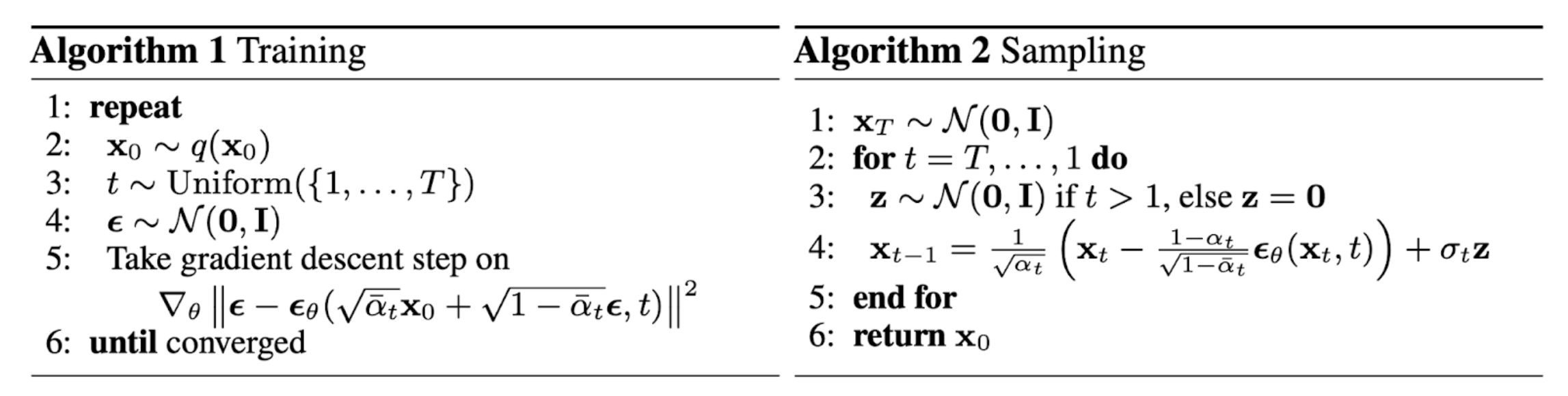 From Lil'Log, originally from Ho et al. Sampling on the right.
We aim to answer 2 questions: Why sampling formula? How to implement it?
Why Sampling Formula?
As we have known from the previous blog, the reverse process is intractable, and the only thing we have is $q(x_{t-1}|x_t, x_0)$. Given the reverse process is Gaussian, it can be expressed as $q(\mathbf{x}_{t-1} \vert \mathbf{x}_t, \mathbf{x}_0) = \mathcal{N}(\mathbf{x}_{t-1}; \tilde{\boldsymbol{\mu}}(\mathbf{x}_t, \mathbf{x}_0), \tilde{\beta}_t \mathbf{I})$.
The reason why we have sampling formula $x_{t-1} = \frac{1}{\sqrt{\alpha_t}} (x_t - \frac{1-\alpha_t}{\sqrt{1-\bar{\alpha}_t}} \epsilon_\theta(x_t, t)) + \sigma_t z$ is that this is exactly the form of revserse Gaussian process of $q(x_{t-1}|x_t, x_0)$!
How to Implement Sampling Formula?
A most naive way of implementing this is do by the formula. There are 2 VERY CRITICAL points to be noted:
- After computing the posterior variance $\sigma_t^2 = \frac{1-\alpha_{t-1}}{1-\alpha_t} \beta_t$, we need to use its square root $\sigma$ instead of $\sigma^2$.
- When sampling, the timesteps are reversed, i.e. mind the loop implementation.
A naive version is as follows:
    def step(
            self,
            current_image,
            model_output: torch.Tensor,
            time_step: int,
        ):
        # get intermediate variables
        batch_size = current_image.shape[0]
        time_step = torch.tensor([time_step] * batch_size).to(current_image.device)
        sqrt_1m_alphas_cumprod_t = extract(self.sqrt_1m_alphas_cumprod, time_step, current_image.shape)
        alphas_t = extract(self.alphas, time_step, current_image.shape)
        alphas_cumprod_t = extract(self.alphas_cumprod, time_step, current_image.shape)
        alphas_cumprod_prev_t = extract(self.alphas_cumprod_prev, time_step, current_image.shape)
        betas_t = extract(self.betas, time_step, current_image.shape)

        posterrior_variance = (1 - alphas_cumprod_prev_t) / (1 - alphas_cumprod_t) * betas_t
        posterrior_variance = torch.clamp(posterrior_variance, min=1e-20)

        print(posterrior_variance.item())

        if time_step != 0:
            z = torch.randn_like(current_image)

        else:
            z = torch.zeros_like(current_image)

        previous_image = (1 / torch.sqrt(alphas_t)) * \
                (current_image - ((1-alphas_t) / (sqrt_1m_alphas_cumprod_t)) * model_output) + \
                (posterrior_variance * z)
        print(f"previous image range:", previous_image.min().item(), previous_image.max().item())
        return previous_image