In this blog we will try to understand the member of diffusion family, DDPM. Given the common structure shared by variational autoencoders (VAEs) and diffusion models, we will first discuss some important content in VAE, and then introduce the DDPM. The blog will try to be self-contained and mathematically clear, but some prior knowledge of VAEs and generative models is assumed.
References:
VAE on Wikipedia
Lil’Log What are Diffusion Models?
STAT940 at University of Waterloo Lecture 17 by Ali Ghodsi
VAE and ELBO
In generative models, our major goal is to look at the dataset, learn the underlying distribution, and then generate new samples from the learned distribution. In the VAE scheme, we employ a structure similar to auto-encoders, which can be seen below:
graph LR
    A[Input] --> B[Encoder]
    B --> C[Latent Space]
    C --> D[Decoder]
    D --> E[Output]
    N((Noise)) --> C
During inference, the encoder is thrown away, we sample some noise to construct a latent variable, and then use the decoder to generate samples. The latent variable is sampled from a prior distribution, usually a standard Gaussian.
I know it might still be unclear, so let’s dive into the math.
Suppose we have some data, we can model the data distribution with a parameter $\theta$. The distribution would be expressed as $p_\theta(x) = p(x|\theta)$. The problem is that we don’t know the parameter $\theta$, and that is exactly what we want to learn. Can we maximize the likelihood of the data? Yes, but it might be hard to optimize well, and we kind of lose the ability to generate new samples.
VAE introduces a latent variable $z$ which models the intricate structure of the data, and it has a joint distribution with data $x$. $p_\theta(x)$ then is a marginal distribution of $p_\theta(x, z)$. We can write the marginal distribution as: $$ p_\theta(x) = \int p_\theta(x, z) dz $$
With simple probability rules, we further write it as: $$ p_\theta(x) = \int p_\theta(x|z)p_\theta(z) dz $$
The underlying assumption here is, the data distribution is controlled by $z$, which is a latent variable with distribution $p_\theta(z)$. Following Bayesian scheme, we have 3 things in the model:
- Prior $p_\theta(z)$
- Likelihood $p_\theta(x|z)$
- Posterior $p_\theta(z|x)$
Typically, we choose the prior to be simple, like a parametrized Gaussian or simply a standard normal distribution, which enables the sampling from it is inexpensive and straightforward. The likelihood $p_\theta(x|z)$ is the probability of a observed data $x$ given latent $z$. It can be easily implemented as a neural network where the input is a latent vector, while the output can be the mean and variance of a normal distribution.
However, the posterior is intractable. To compute it, we need to apply Bayes’s theorm: $$ p_\theta(z|x)=\frac{p_\theta(x|z)p_\theta(z)}{p_\theta(x)} $$ Clearly, we don’t know about the $p_\theta(x)$. While this is a sad new, we further introduce a function $q_\phi(z|x)\approx p_\theta(z|x)$ to approximate posterior using a different set of parameters $\phi$. Notice that this is not a design comes from nowhere, instead it comes from the Evidence Lower Bound (ELBO) inequality for general latent variable models!
    graph LR
    Z((z)) --likelihood-->X((x))
    X((x)) --posterior--> Z
So what is ELBO? ELBO gives a way to do maximize likelihood estimation (MLE) even when the $p_\theta(z|x)$ is intractable. We can derive ELBO from MLE on $p_\theta(x)=log p(x|\theta)$.
$$ \begin{aligned} \log p(x|\theta) &= \log \int p(x, z |\theta) dz \\ &= \log \int p(x, z |\theta) \frac{q(z|x, \phi)}{q(z|x, \phi)} dz\\ &= \log \mathbb{E}_{z \sim q(\cdot|x,\phi)} \left[ \frac{p(x, z | \theta)}{q(z|x, \phi)} \right] \\ &\geq \mathbb{E}_{z \sim q(\cdot|x,\phi)} \left[ \log \frac{p(x, z | \theta)}{q(z|x, \phi)} \right] \quad \text{(Jensen’s Inequality)} \end{aligned} $$
The ELBO can be further decomposed into $$ \begin{aligned} & \ \mathbb{E}_{z \sim q(\cdot|x,\phi)} \left[ \log \frac{p(x, z | \theta)}{q(z|x, \phi)} \right]\\ & =\mathbb{E}_{z \sim q(\cdot|x,\phi)} \left[ \log \frac{p(x, z | \theta)}{q(z|x, \phi)} \right]\\ & = \mathbb{E}_{z \sim q(\cdot|x,\phi)} \left[ \log \frac{p(x|z, \theta)p(z|\theta)}{q(z|x, \phi)} \right]\\ & = \mathbb{E}_{z \sim q(\cdot|x,\phi)} \left[ \log p(x|z, \theta) + \log \frac{p(z|\theta)}{q(z|x, \phi)} \right]\\ & = \mathbb{E}_{z \sim q(\cdot|x,\phi)} \left[ \log p(x|z, \theta) \right] - \mathbb{E}_{z \sim q(\cdot|x,\phi)} \left[ \log \frac{q(z|x, \phi)}{p(z|\theta)} \right]\\ & = \mathbb{E}_{z \sim q(\cdot|x,\phi)} \left[ \log p(x|z, \theta) \right] - D_{KL}(q_\phi(z|x)||p_\theta(z)) \end{aligned} $$
It is good to remember here that, the KL divergence between 2 distributions is: $$ D_{KL}(q||p) = \int q(x) \log \frac{q(x)}{p(x)} dx\\ D_{KL}(q||p) = \mathbb{E}_{x\sim q(\cdot)}[\log \frac{q(x)}{p(x)}] $$
We can maximize this lower bound to maximize the log likelihood of the data, but still, not very convenient. So in real implementation, we maximize the following equivalent one: $$ L_{\theta, \phi}(x) = \mathbb{E}_{z\sim q_\phi(\cdot|x)}[\log p_\theta(x|z)] - D_{KL}(q_\phi(\cdot|x)||p_\theta(\cdot)) $$
Given the foresay model, which learns the distribution and gives a way to generate new sample, we need to find a way to learn parameters. For VAE, there are 2 things we want to optimize:
- We want the re-construction to be precise. Given the data $x_i$, we can compute the corresponding latent variable $z_i$, and the decoder should be able to precisely give me $x_i$ given $z_i$
- We want the approximation $q_\phi(z|x)\approx p_\theta(z|x)$ to be accurate, otherwise the latent variable generated form training data would be nonsense.
The 2 terms we optimize corresponds to the 2 target we want to optimize. As we model the latent $p_\theta(z)$ to be normal Gaussian and the $q_\phi(z|x)$ to be Gaussian as well, the KL divergence have closed form expression. Notice that $q_\phi(z|x)$ is implemented through reparametrization trick, but we will skip it here and focuse more on the diffusion part.
DDPM: the Overview
What is the common style of generative models? Build a network that takes in some randomness and generate new data similar to those in training set. Diffusion models are also employing this style. During inference, it takes a noise (like a purely noisy image), and step-by-step denoise the image, and reveal the data.
    flowchart LR
    A[x0] -->|Noise| B[x1]
    B -->|Noise| C[x2]

    C -->|Noise| D[...]
    D -->|Noise| E[xT]

    E -->|Denoise| D
    D -->|Denoise| C
    C -->|Denoise| B
    B -->|Denoise| A[x0]

    classDef noising fill:#f9f,stroke:#333,stroke-width:2px;
    classDef denoising fill:#9ff,stroke:#333,stroke-width:2px;
    class A,B,C,D,E,F noising,denoising;
We will discuss the DDPM in the following sections with image as the type of our data.
DDPM: Forward Process
The forward process of DDPM does not involve learning. It is simply a process that iteratively add noise into the data. The process is as follows:
- Start with a image $x_0$
- Add noise into the image to get $x_1$ by $x_1 = \sqrt{1-\beta_t} x_0 + \sqrt{\beta_t} \epsilon_t$, where $\epsilon_t \sim \mathcal{N}(0, I)$ and the sequence of $\beta_t$ is previously defined
- Repeat the process until $x_T$ is obtained. So $x_t = \sqrt{1-\beta_t} x_{t-1} + \sqrt{\beta_t} \epsilon_t$
- The final image $x_T$ is the noisy image we want to denoise.
In the forward process, we have a nice property that gives any $x_t$ directly without repeat the above process. First we let $\alpha_t = 1-\beta_t$ and $\bar{\alpha}_t = \prod_{i=1}^t \alpha_i$. Then we can write $x_t$ as: $$ \begin{aligned} x_t &= \sqrt{\alpha_t}x_{t-1} + \sqrt{1-\alpha_t}\epsilon_{t-1}\\ &= \sqrt{\alpha_t\alpha_{t-1}}x_{t-2} + \sqrt{1-\alpha_t\alpha_{t-1}}\epsilon_{t-2}\quad \text{; merge 2 Gaussians}\\ &=\cdots\\ &= \sqrt{\bar{\alpha}_t}x_0 + \sqrt{1-\bar{\alpha}_t}\epsilon_0 \end{aligned} $$
We can write it down as a transition probability: $$ q(x_t|x_0) = \mathcal{N}(x_t|\sqrt{\bar{\alpha}_t}x_0, (1-\bar{\alpha}_t)I) $$
In this manner, we can easily sample any data and construct the noisy image at timestep $t$.
DDPM: Reverse Process
Forward process is easy, while reverse process give DDPM the ability to generate. Here is a general idea of the reverse process:
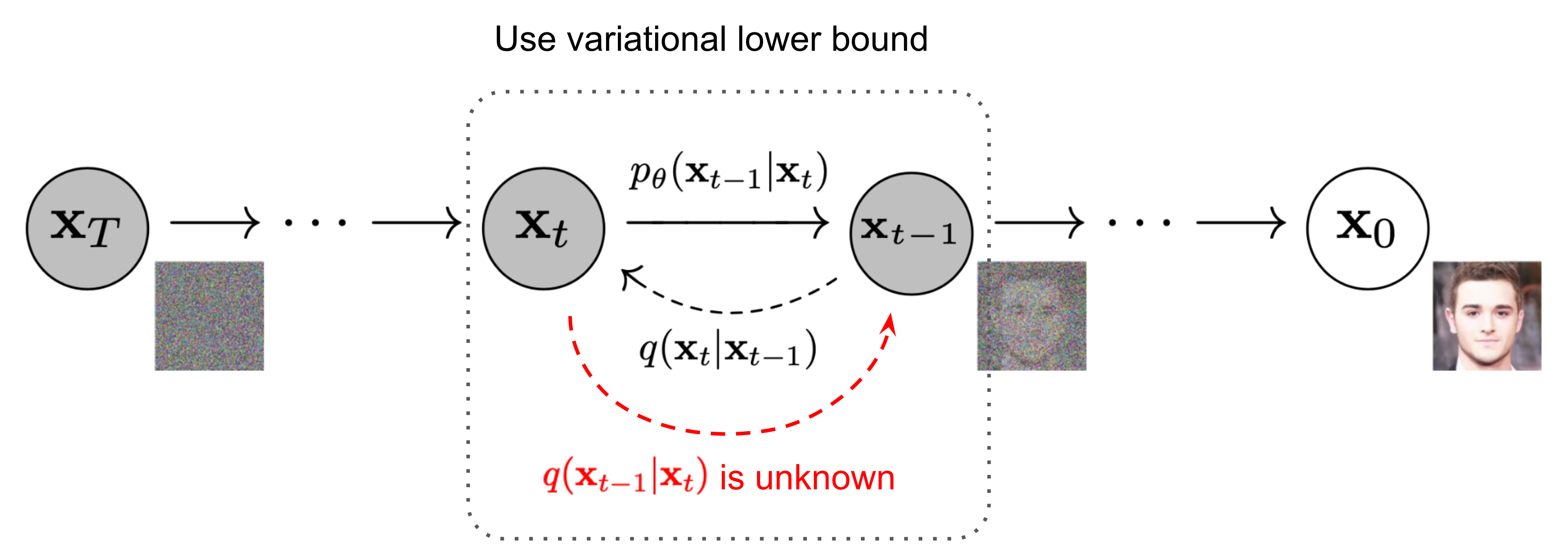 From Lil'Log, originally from Ho et al. Already look a little bit like VAE.
Previously, we established the forward process with transition probability: $$ q(x_t|x_{t-1}) = \mathcal{N}(x_t|\sqrt{\alpha_t}x_{t-1}, (1-\alpha_t)I) $$
The reverse process aims to revert the process with $q(x_{t-1}|x_t)$ so we can sample a noise as $x_T$ and generate the clear image by repeatedly sampling $x_{t-1}$ from $x_t$. Notice that, if the $\beta_t$ is small enough, $q(x_{t-1}|x_t)$ is Gaussian.
If we view the one single step in the above image as a VAE (latent variable is $x_{t-1}$), we can see that $q(x_{t-1}|x_t)$ is intractable just like $p(z|x, \theta)$ in VAE. However, we may still follow the scheme of VAE and write down the likelihood: $$ p_\theta(x_{0:T}) = p(x_T)\prod_{t=1}^T p(x_{t-1}|x_{t})\\ p(x_{t-1}|x_{t}) = \mathcal{N}(x_{t-1}|\mu_\theta(x_t, t), \Sigma_\theta(x_t, t)) $$
The first line is the likelihood of an entire sequence of noising process. As we have said, the reverse process $p(x_{t-1}|x_{t})$ is intractable, so we need to think of the other way. The reverse conditional probability is tractable when conditioned on $x_0$.
This is a tricky part. There are 2 questions to answer: Why is it tractable? How to understand it?
- The tractable form would be $q(x_{t-1}|x_t, x_0)$, which is similar to the other $q$ we use in VAE. Mathematically, when given $x_0$, the forward process $q(x_t|x_{t-1}, x_0)=q(x_t|x_{t-1})$, and it is a Gaussian process. The reverse process is Gaussian as well, and it can be derived directly from Bayes’ theorem. The tractable form is: $$ q(x_{t-1}|x_t, x_0) = \mathcal{N}(x_{t-1}|\mu(x_t, t), \Sigma(x_t, t)) $$
- The understanding part is a little bit tricky. Given $x_0$, we can think of having an oracle view on the whole diffusion process, and thus we can easily sample $x_{t-1}$ given $x_t$ (just by look at one timestep before). The $x_0$ is like a “context” that helps us to sample $x_{t-1}$.
Now we can write down the likelihood of the entire sequence as (with $x_0$ as the context): $$ \begin{aligned} q(x_{t-1}|x_t, x_0) &= \mathcal{N}(x_{t-1}| \tilde{\mu}_\theta(x_t, x_0), \tilde{\beta_t}I)\\ &\text{not cosider the std for DDPM} \end{aligned} $$
Now our target is to train the neural network to learn the probability for reverse process. To do so, we need to derive the objective function to optimize the network. As we have said before, the process is similar to VAE, which is maximizing the lighlihood of the data.
For VAE: $$ \log p_\theta(x) \geq \mathbb{E}_{z\sim q_\phi(\cdot|x)}[\log p_\theta(x|z)] - D_{KL}(q_\phi(z|x)||p_\theta(z)) $$
Similarly, we consider $x_{1:T}$ as the hidden variable. But notice that in VAE both $p$ and $q$ are parametrized and trained, while in DDPM the process from $x_0$ (data) to $x_{1:T}$ is known by the forward process. So we don’t have a parametrized $q$ in DDPM. $$ \log p_\theta(x_0) \geq \mathbb{E}_{x_{1:T}\sim q(\cdot|x_{0})}[\log p_\theta(x_{0}|x_{1:T})] - D_{KL}(q(x_{1:T}|x_0)||p_\theta(x_{1:T})) $$
And this lower bound is what we want to maximize, and we further transform the lower bound into the tractable form for implementation. Let’s kind of reverse our derivation for variational lower bound: $$ \begin{aligned} &\ \mathbb{E}_{x_{1:T}\sim q(\cdot|x_{0})}[\log p_\theta(x_{0}|x_{1:T})] - D_{KL}(q(x_{1:T}|x_0)||p_\theta(x_{1:T}))\\ & = \mathbb{E}_{x_{1:T}\sim q(\cdot|x_{0})}[\log p_\theta(x_{0}|x_{1:T})] + \mathbb{E}_{x_{1:T}\sim q(\cdot|x_{0})}[\log \frac{q(x_{1:T}|x_0)}{p_\theta(x_{1:T})}]\quad \text{; KL}\\ & = \mathbb{E}_{x_{1:T}\sim q(\cdot|x_{0})}[\log p_\theta(x_{0}|x_{1:T}) - \log \frac{q(x_{1:T}|x_0)}{p_\theta(x_{1:T})}]\quad \text{; merge 2 exp}\\ & = \mathbb{E}_{x_{1:T}\sim q(\cdot|x_{0})}[\log p_\theta(x_{0}|x_{1:T}) + \log \frac{p_\theta(x_{1:T})}{q(x_{1:T}|x_0)}]\quad \text{; log rule}\\ & = \mathbb{E}_{x_{1:T}\sim q(\cdot|x_{0})}[\log \frac{p_\theta(x_{0}| x_{1:T})p_\theta(x_{1:T})}{q(x_{1:T}|x_0)}]\quad \text{; log rule}\\ & = \mathbb{E}_{x_{1:T}\sim q(\cdot|x_{0})}[\log \frac{p_\theta(x_{0:T})}{q(x_{1:T}|x_0)}]\quad \text{; basic probability}\\ \end{aligned} $$
Now we have some concise expression, and we want to decompose the trajectory part inside. $$ \begin{aligned} &\ \mathbb{E}_{x_{1:T}\sim q(\cdot|x_{0})}[\log \frac{p_\theta(x_{0:T})}{q(x_{1:T}|x_0)}]\\ & = \mathbb{E}_{x_{1:T}\sim q(\cdot|x_{0})}[\log \frac{p(x_{T})\prod_{t=1}^{T}p_\theta(x_{t-1}|x_t)}{q(x_{1:T}|x_0)}]\\ & = \mathbb{E}_{x_{1:T}\sim q(\cdot|x_{0})}[\log p(x_{T}) + \sum_{t=1}^{T}\log p_\theta(x_{t-1}|x_t) - \log q(x_{1:T}|x_0)]\\ & = \mathbb{E}_{x_{T}\sim q(\cdot|x_{0})}[\log p(x_{T})] + \sum_{t=1}^{T}\mathbb{E}_{x_{t-1}\sim q(\cdot|x_t, x_0)}[\log p_\theta(x_{t-1}|x_t)] \\ & - \mathbb{E}_{x_{1:T}\sim q(\cdot|x_{0})}[\log q(x_{1:T}|x_0)]\\ & = \mathbb{E}_{x_{T}\sim q(\cdot|x_{0})}[\log p(x_{T})] + \sum_{t=1}^{T}\mathbb{E}_{x_{t-1}\sim q(\cdot|x_t, x_0)}[\log p_\theta(x_{t-1}|x_t)] \\ & - \mathbb{E}_{x_{1:T}\sim q(\cdot|x_{0})}[\log \prod_{t=1}^{T}q(x_t|x_{t-1}, x_0)]\\ & = \mathbb{E}_{x_{T}\sim q(\cdot|x_{0})}[\log p(x_{T})] + \sum_{t=1}^{T}\mathbb{E}_{x_{t-1}\sim q(\cdot|x_t, x_0)}[\log p_\theta(x_{t-1}|x_t)] \\ & - \sum_{t=1}^{T}\mathbb{E}_{x_{t}\sim q(\cdot|x_{t-1}, x_0)}[\log q(x_t|x_{t-1})] \end{aligned} $$
Now we keep the first term and merge the summation of the second term and the third term: $$ \begin{aligned} &\ \mathbb{E}_{x_{T}\sim q(\cdot|x_{0})}[\log p(x_{T})] + \sum_{t=1}^{T}\mathbb{E}_{x_{t-1}\sim q(\cdot|x_t, x_0)}[\log p_\theta(x_{t-1}|x_t)] \\ & - \sum_{t=1}^{T}\mathbb{E}_{x_{t}\sim q(\cdot|x_{t-1}, x_0)}[\log q(x_t|x_{t-1})]\\ & = \mathbb{E}_{x_{T}\sim q(\cdot|x_{0})}[\log p(x_{T})] + \sum_{t=1}^{T}\mathbb{E}_{x_{t-1}\sim q(\cdot|x_t, x_0)}[\log p_\theta(x_{t-1}|x_t) - \log q(x_t|x_{t-1})]\\ & = \mathbb{E}_{x_{T}\sim q(\cdot|x_{0})}[\log p(x_{T})] + \sum_{t=1}^{T}\mathbb{E}_{x_{t-1}\sim q(\cdot|x_t, x_0)}[\log \frac{p_\theta(x_{t-1}|x_t)}{q(x_t|x_{t-1})}]\quad \text{; KL} \end{aligned} $$
The intuition here is to make the backward process to mimic the forward process. The KL divergence term is to make the reverse process to be close to the forward process. And we have talked about the tractable form problem and we see the above thing is not tractable. So add condition on $x_0$ and we can get the tractable form. $$ q(x_{t-1}|x_t) = q(x_{t-1}|x_t, x_0) = \frac{q(x_{t-1}, x_t|x_0)}{q(x_t|x_0)}; \quad \text{Bayes’ Theorem} $$
Plug this into the above equation, we can get the tractable form of the objective function. The final form is: $$ \begin{aligned} \mathcal{l}(x_0) &= \mathbb{E}_{x_{1:T}\sim q(\cdot|x_t, x_{0})}[\log p(x_{T}) \\ & + \sum_{t=2}^{T}\log \frac{p_\theta(x_{t-1}|x_t)}{q(x_{t-1}|x_t, x_0)} + \sum_{t=2}^{T}\log \frac{q(x_{t-1}| x_0)}{q(x_t|x_0)} + \log \frac{p_\theta(x_{0}|x_1)}{q(x_{1}|x_0)}] \end{aligned} $$
We can cancel many things in the term $\sum_{t=2}^{T}\log \frac{q(x_{t-1}| x_0)}{q(x_t|x_0)}$ and the final form after cancellation is $-\log q(x_T|x_0) + \log q(x_1|x_0)$.
The Ultimate negative ELBO becomes: $$ \begin{aligned} -\mathcal{l}(x_0) &= -\mathbb{E}_{x_{1:T}\sim q(\cdot|x_t, x_{0})}[\log p(x_{T}) \\ & + \sum_{t=2}^{T}\log \frac{p_\theta(x_{t-1}|x_t)}{q(x_{t-1}|x_t, x_0)} + \log \frac{p_\theta(x_{0}|x_1)}{q(x_{1}|x_0)}]\\ & = D_{KL}(q(x_T|x_0)||p(x_T))\quad \text{; Ignored, constant}\\ & + \sum_{t=2}^{T}\mathbb{E}_{x_t \sim q(\cdot|x_t, x_0)}D_{KL}(q(x_{t-1}|x_t, x_0)||p_\theta(x_{t-1}|x_t))\quad \text{; t-1 Loss}\\ & + \mathbb{E}_{x_1\sim q(\cdot|x_0)}\log p_\theta(x_0|x_1) \quad \text{; 0-1 Loss} \end{aligned} $$
Quick Summary! so far we have experienced some math, and essentially, we have:
- ELBO for DDPM viewing $x_{1:T}$ as hidden variable
- Decompose the $1:T$ sequence into discrete parts
- Simplified the expression
- Plug in the condition on $x_0$ so we have a tractable form
Now we go back to the loss derivation. First we look at the KL divergence, and one thing we now know is $q(x_{t-1}|x_t, x_0)$ is tractable and it can be obtained through god-level high-school algebra (see here). The takeaway is $q(x_{t-1}|x_t, x_0)$ is Gaussian with mean $\bar{\mu}_t = \frac{1}{\alpha_t}(x_t - \frac{1-\alpha_t}{\sqrt{1-\bar{\alpha}_t}}\epsilon_t)$, where $\epsilon_t \sim \mathcal{N}(0, I)$ and $\bar{\alpha}_t = \prod_{i=1}^t \alpha_i$.
The KL divergence term is then the KL divergence between distribution $q(x)=\mathcal{N}(x|\mu_q, \Sigma_q)$ and $p(x)=\mathcal{N}(x|\mu_p, \Sigma_p)$, where for $p$ the mean is $\mu_\theta(x_t, t)=\frac{1}{\sqrt{\alpha_t}}(x_t - \frac{1-\alpha_t}{\sqrt{1-\bar{\alpha}_t}}\epsilon_\theta(x_t, t))$.
The loss function is then: $$ \begin{aligned} &\ L_t \\ &= \mathbb{E}_{\mathbf{x}_0, \boldsymbol{\epsilon}} \Big[\frac{1}{2 | \boldsymbol{\Sigma}_\theta(\mathbf{x}_t, t) |^2_2} | \color{blue}{\tilde{\boldsymbol{\mu}}_t(\mathbf{x}_t, \mathbf{x}_0)} - \color{green}{\boldsymbol{\mu}_\theta(\mathbf{x}_t, t)} |^2 \Big] \\ &= \mathbb{E}_{\mathbf{x}_0, \boldsymbol{\epsilon}} \Big[\frac{1}{2 |\boldsymbol{\Sigma}_\theta |^2_2} | \color{blue}{\frac{1}{\sqrt{\alpha_t}} \Big( \mathbf{x}_t - \frac{1 - \alpha_t}{\sqrt{1 - \bar{\alpha}_t}} \boldsymbol{\epsilon}_t \Big)} - \color{green}{\frac{1}{\sqrt{\alpha_t}} \Big( \mathbf{x}_t - \frac{1 - \alpha_t}{\sqrt{1 - \bar{\alpha}_t}} \boldsymbol{\boldsymbol{\epsilon}}_\theta(\mathbf{x}_t, t) \Big)} |^2 \Big] \\ &= \mathbb{E}_{\mathbf{x}_0, \boldsymbol{\epsilon}} \Big[\frac{ (1 - \alpha_t)^2 }{2 \alpha_t (1 - \bar{\alpha}_t) | \boldsymbol{\Sigma}_\theta |^2_2} |\boldsymbol{\epsilon}_t - \boldsymbol{\epsilon}_\theta(\mathbf{x}_t, t)|^2 \Big] \\ &= \mathbb{E}_{\mathbf{x}_0, \boldsymbol{\epsilon}} \Big[\frac{ (1 - \alpha_t)^2 }{2 \alpha_t (1 - \bar{\alpha}_t) | \boldsymbol{\Sigma}_\theta |^2_2} |\boldsymbol{\epsilon}_t - \boldsymbol{\epsilon}_\theta(\sqrt{\bar{\alpha}_t}\mathbf{x}_0 + \sqrt{1 - \bar{\alpha}_t}\boldsymbol{\epsilon}_t, t)|^2 \Big] \end{aligned} $$
The author further simplify the loss function and the final form is: $$ \begin{aligned} L_t^\text{simple} &= \mathbb{E}_{t \sim [1, T], \mathbf{x}_0, \boldsymbol{\epsilon}_t} \Big[|\boldsymbol{\epsilon}_t - \boldsymbol{\epsilon}_\theta(\mathbf{x}_t, t)|^2 \Big] \\ &= \mathbb{E}_{t \sim [1, T], \mathbf{x}_0, \boldsymbol{\epsilon}_t} \Big[|\boldsymbol{\epsilon}_t - \boldsymbol{\epsilon}_\theta(\sqrt{\bar{\alpha}_t}\mathbf{x}_0 + \sqrt{1 - \bar{\alpha}_t}\boldsymbol{\epsilon}_t, t)|^2 \Big] \end{aligned} $$
The final training looks like in this image:
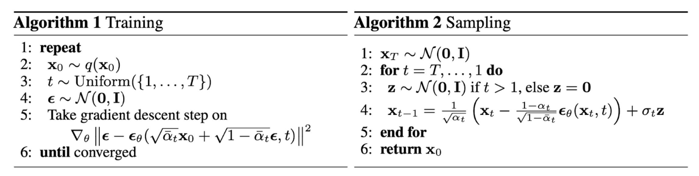 From Lil'Log, originally from Ho et al.
DDPM: Inference
The inference process is simple. We have the forward process, and we can sample the noise at $x_T$ and then generate the clear image by repeatedly sampling $x_{t-1}$ from $x_t$.